The topological fingerprint was introduced in [1] and motivated by [2]; for various applications see also [3]. It was successfully used to describe entanglement of all proteins [4] deposited in the PDB. Herein, we used it to describe the crucial information about the topology of the given chromosome structure. The fingerprint encodes information about locations of the "knot core", "knot tails", "slipknot loops", and "slipknot tails", whose definitions are given below.
The knotting fingerprint takes a form of a matrix diagram by using the procedure established by us before for proteins [4]. The matrix diagram is constructed as follows. For a given chain of length N, all its subchains spanning between residues k and l (for 1≤k<l≤N) are analyzed. If a subchain from k to l is knotted (as determined by the analysis described in section Knot detection), then a point with coordinates (k,l) is denoted in relevant color in a plot. For example, points representing knots 31, 41, 51, 52, 62, 63, 76 are respectively green, red, orange, grey, violet. All more complex knots are shown with different shades of grey. The intensity of a color represents a probability of detecting a given knot (knots are detected only with some probability, which is a consequence of a choice of its closure to a closed loop, as explained in section Knot detection). The figure below presents an example of a knotting fingerprint, which in this case contains areas representing a knot and two types of slipknots.
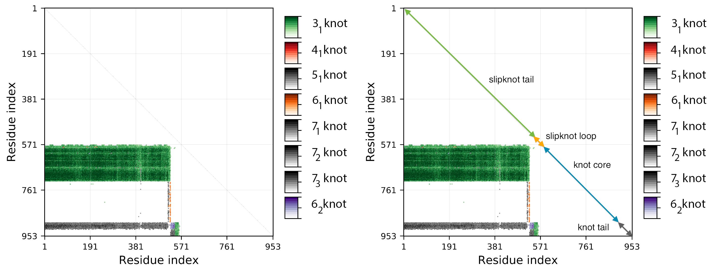
Fig. 1 Left panel example of a knotting fingerprint with S3151624176886352820 topological notation detected in chromosome o, model 01, cell 1 [5]. The matrix arises from the random closure method (20 randomly selected points on the sphere). The right panel shows the location of the knot core, knot tails, slipknot tail and slipknot loop for the sample slipknot of type 31. Please note that only the knot with the highest probability is shown.
In a given knot or slipknot several geometric elements can be distinguished. These elements are denoted in different colors along the diagonal of the matrix diagram as shown schematically in the figure below:
The matrix diagram is interactive: after choosing a knot type (if more than one knot type is detected) from the table, the data corresponding to this knot is shown in the diagram Fig. 2. By default the data corresponding to the knot formed by the whole chain (for knotted chromosomes), or the most complicated slipknot (for chromosomes with slipknots) is shown in the diagram.
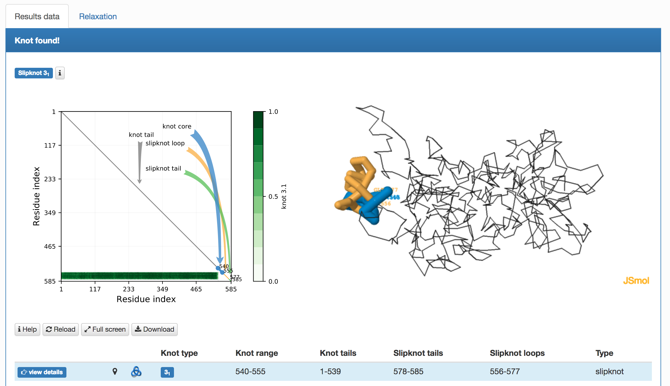
Fig. 2 An example for the data presentation for a slipknotted chromosome. In this example the analysis reveals that the entire analyzed chain (chromosome r, model 01, cell 1 [4]) forms an unknot and has a subchain forming a 31 knot. Diagram in the top left: knotting fingerprint revealing the positions of the subchain forming a 31 knot. Top right: graphical representation of the chromosome in JSmol, with the knot core, slipknot and knot tails highlighted in various colors (knot core in blue, slipknot loop in orange, and the knot tail in grey). In grey the knot tail is shown. In the middle left buttons: iHelp - description how to use JSmol, Reload of data and Download - SVG maps and PNG map. Table at the bottom: detailed data about knots and slipknots formed by backbone subchains.
Fig. 3 presents the fingerprint of chromosome o, model 1, cell 1 determined based on three different closure methods: centre of mass, random closure and direct closure.
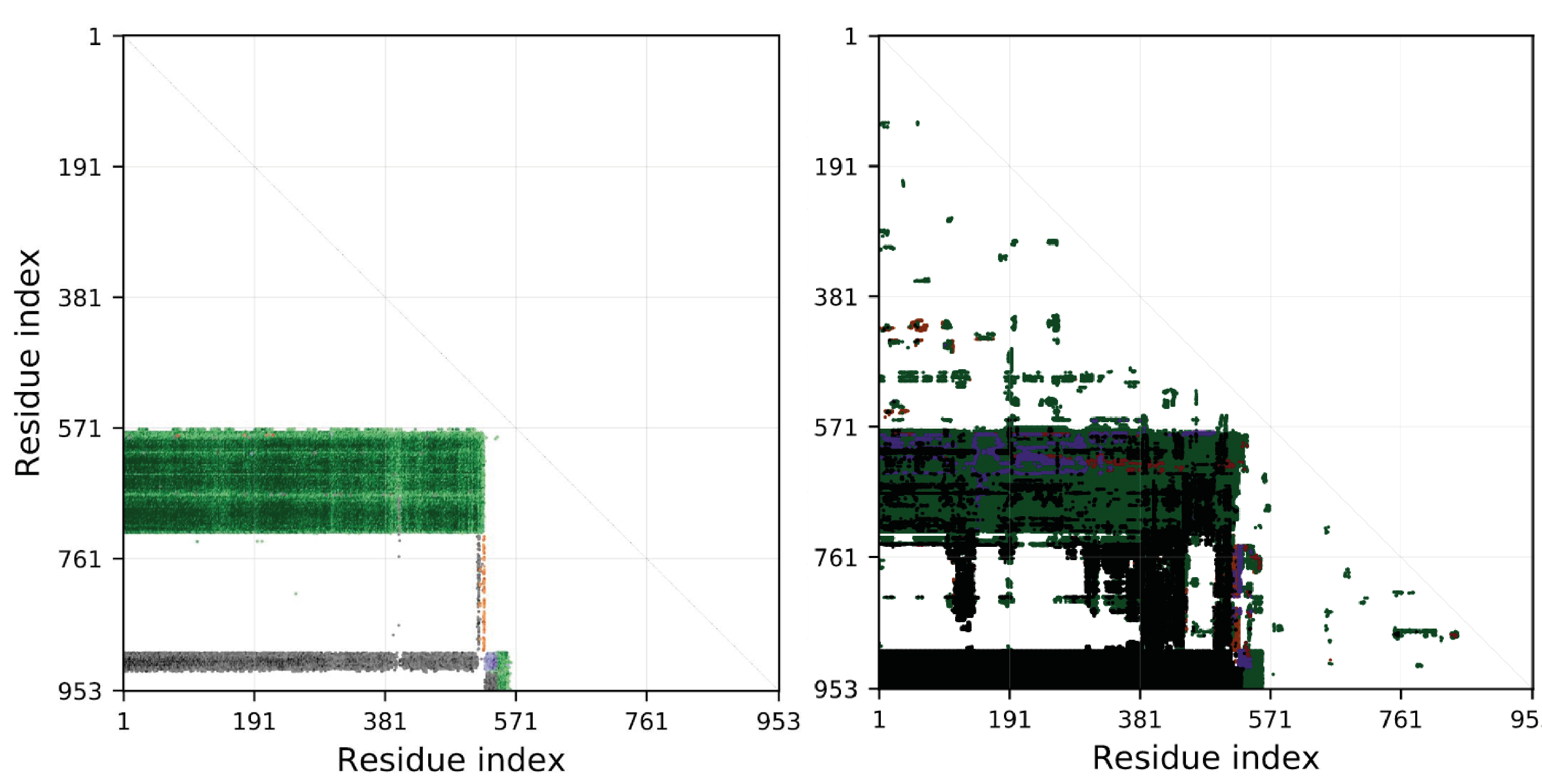
Fig. 3 Fingerprint for chromosome o, model 1, cell 1 determined based on three different closure methods: centre of mass, random closure and direct closure, respectively
Remark 1: Please note that topological fingerprints based on the current available data [5] is usually much more complicated than this presented on the Fig. 1.
Remark 2: In the case of the random closure method, to speed up the time of calculation, the fingerprint is determined for every seventh configuration.