The user can upload and analyze two types of data: either a single chromosome, or a whole cell. In this section we explain how to identify entanglement between a pair of chromosomes. This analysis can be conducted based on random, centre of mass, or direct closure method. Entanglement of links is also computed by Gaussian linking integral, which is another measure of entanglement between a pair of chromosomes. Moreover, the user can use all these methods together with the relaxation procedure to estimate entanglement stability [1].
Entanglement of a pair of chromosome is presented in the following manner. The information displayed from top to bottom of the result page can be divided into:
Each of these parts is described in detail below. Additional examples are shown here - examples.
At the top of the page, the first tab indicates the status of a submitted job. The tab summarizes options used by the user to submit a job and current job performance. All this information is described here
Comprehensive information about an entanglement of a pair of chromosomes is presented using three interactive matrices as shown in Fig. 1.
Let us remind that Max |GLN| is equal max{maxGLN-minGLN}, where minGLN and maxGLN denote respectively minimum and maximum values of GLN between a chromosome 1 and any fragment of a chromosomes 2, and a chromosome 2 and any fragment of a chromosomes 1.
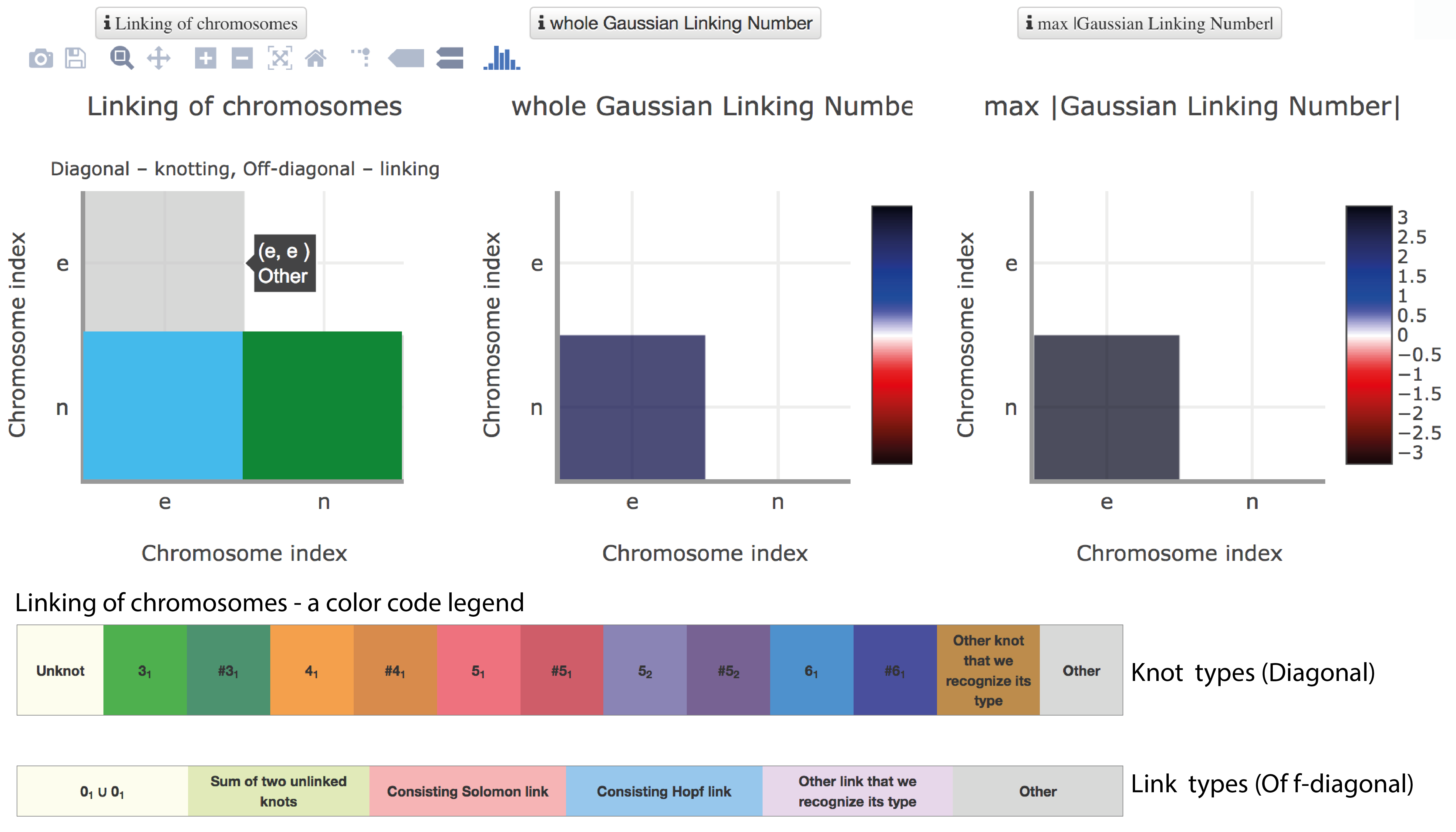
Fig. 1 Overview of a comprehensive analysis of a pair of chromosomes, first part of an example page. Left: the interactive matrix - Linking chromosomes - showing with color code identified knots, links. The color code used in the Knot Gnome is shown below the matrix. Midle and right: interactive matrices to shows entanglement computed based on Gaussian linking integral, which is another measure of entanglement between a pair of chromosomes. The definition of whGLN and max|GLN| is provided here. Upon pointing the cursor on the element of matrix detail information about topology is provided. Upon clicking on the element of matrix a new webpage will be provided containing the Graphical representation of the chromosomes and knot or link likelihood, and the more extended version of the knot or link table is displayed. All matrices can be e.g. zoom in/out, modified and save using open source tool Plotly which allows interactive data visualization (https://plot.ly/).
The topological and structural details about the knot or the most probable knot (in the case of probabilistic method) are stored in the table below three the matrices (Fig. 1). Each row of the table describes knotting on a single chromosome chain. By default the chromosomes with a trivial topology are not shown in the table, they are listed in the table by clicking the button "Toggle hidden" above the table. In each row, one can find the miniature depiction of the identified knot along with its name and probability. Upon clicking on View details - located in the left-most part of the table - a new website is provided which contains the Graphical representation of the chromosomes, knot likelihood, and the knot table. This content is the same as in the case of the Main type knot analysis and is described here. When probabilistic method is used, this table contains other types of knots identified for this chromosome not presented in the main page.
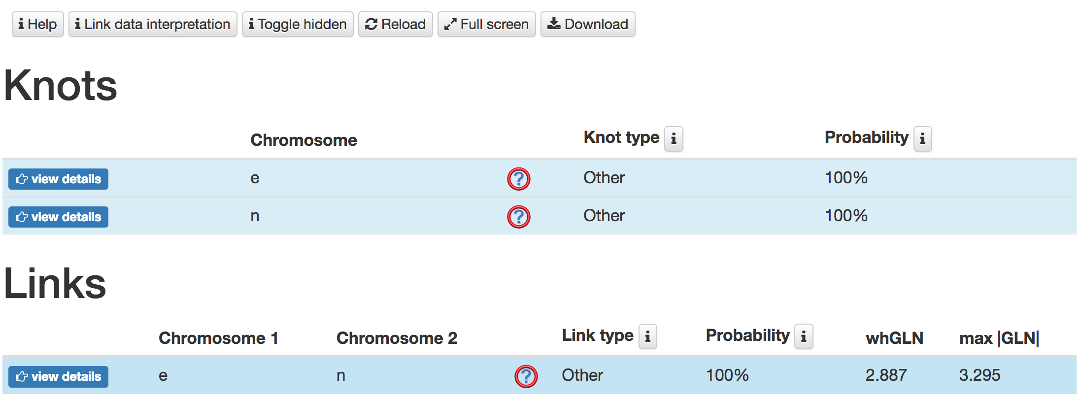
Fig. 2 Tables showing indentified knots and link in analyzed exemplary pair of chromosomes. Tables contains the types entanglement, schematic drawing of topology, probability and entanglement measured with Gaussian Linking Number - whGLN, max|GLN|. Upon clicking on "view details" a new webpage including the Graphical representation of the chromosomes and the knot or link likelihood, and the more extended version of the knot or link table will appear. Presented data were analyzed with the centre of mass method. Above the tables are places additional buttons to facilitated further analysis. The button "Toggle hidden" should be use to include in the tables trivial topologies. The download button allows downloading all topological information about the investigated structures presented in the tables, to perform own analysis.
The topological and structural details about the most probable type of link are stored in the table (Fig. 2), below the matrices (Fig. 1). Each row of the table (when only one pair is analyzed table contains one row) describes linking between a pair of chromosomes. In each row, one can find the miniature depiction of the link identified along with its name and probability, values of whGLN and max|GLN|. Upon pointing the cursor on max|GLN| the user can see the range of atoms corresponding to the shortest fragments of the chromosomes which wind around each other (for details see GLN description). Upon clicking on View details - located in the left-most part of the table - a new website is provided with the graphical presentation of chromosomes and link likelihood, and the link table. This subpage is described here. Composition of these information on the one website allows user to verified (e.g. results of closure method) and understand better topological analysis. When the random closure method is used this table contains also other types of identified links - not only the most probability link.
Details about indentified links are presented on subpage which contains the JSmol presentation of the chromosomes structures (left) and the pie chart (right) representing the likelihood of each link identified. By default the most probable link type is show in the center of the pie chart.
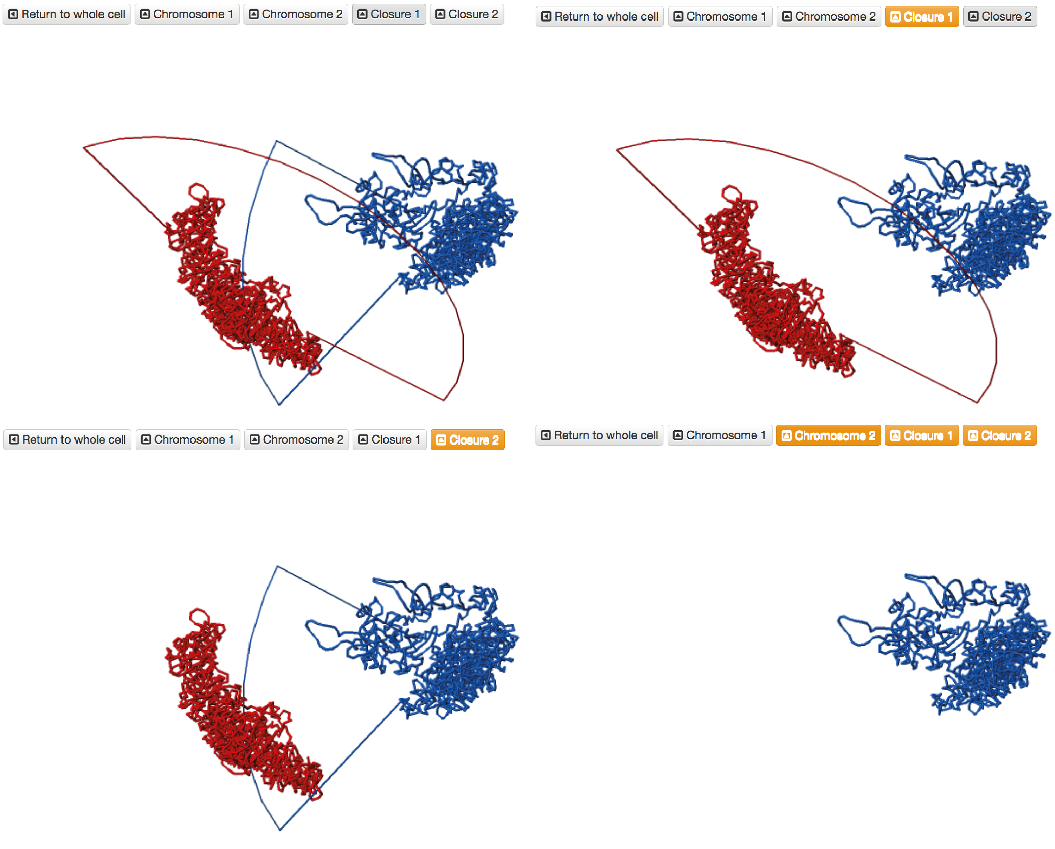
Fig. 3 An example of chromosomes structures presentation using JSmol applet when the deterministic method is used. These chromosomes are unlinked, however, each single chromosome forms a 31 knot.
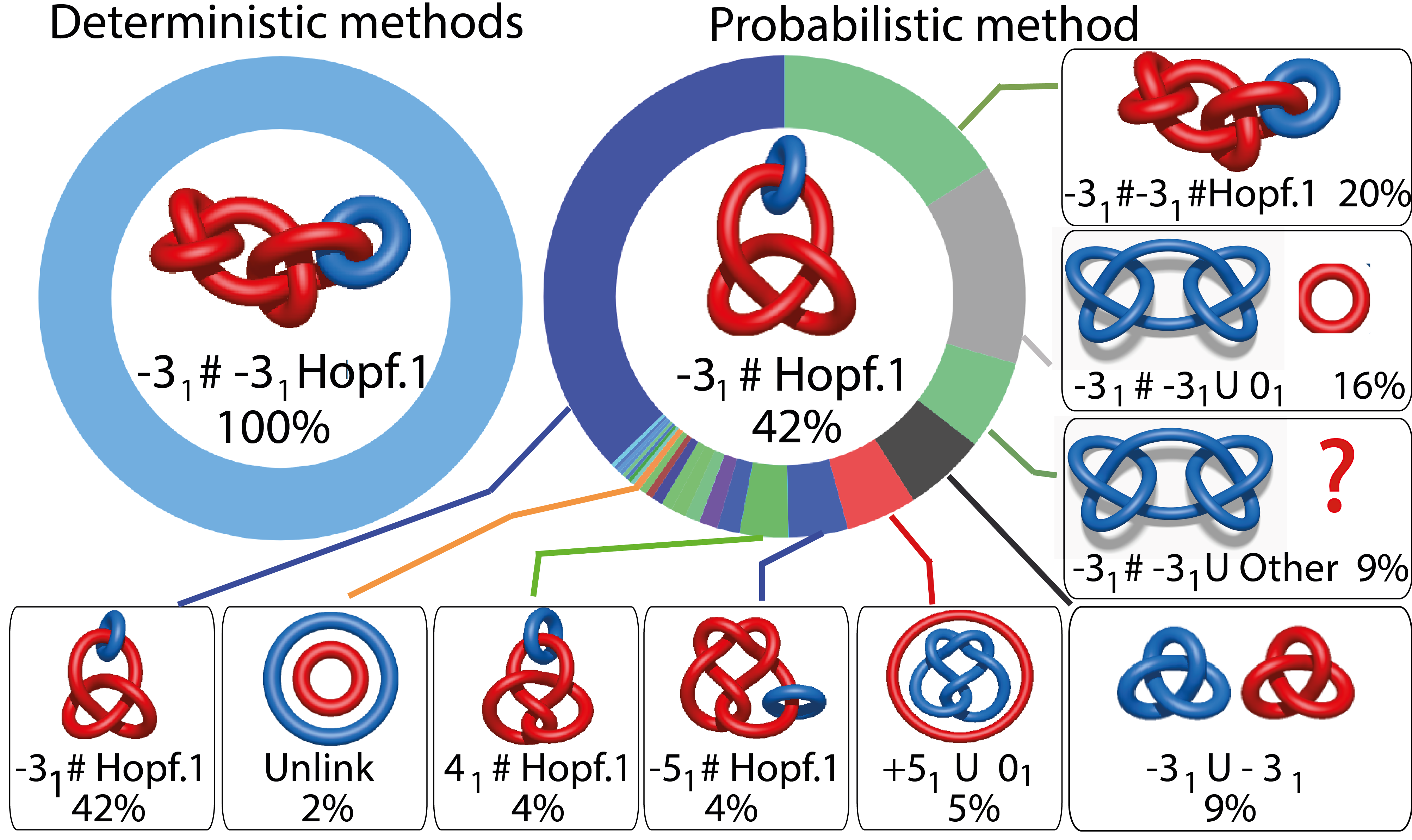
Fig. 4 The pie chart representing the likelihood of the links identified. Left, an example of a pie chart when the deterministic closure methods are used. Right, an example of a pie chart when random closure method is used. In the case of random closure method by default, the most probable link is shown in the center of the plot. Upon placing the cursor over a region of the chart, the corresponding link and its likelihood are displayed in the center of the pie chart.
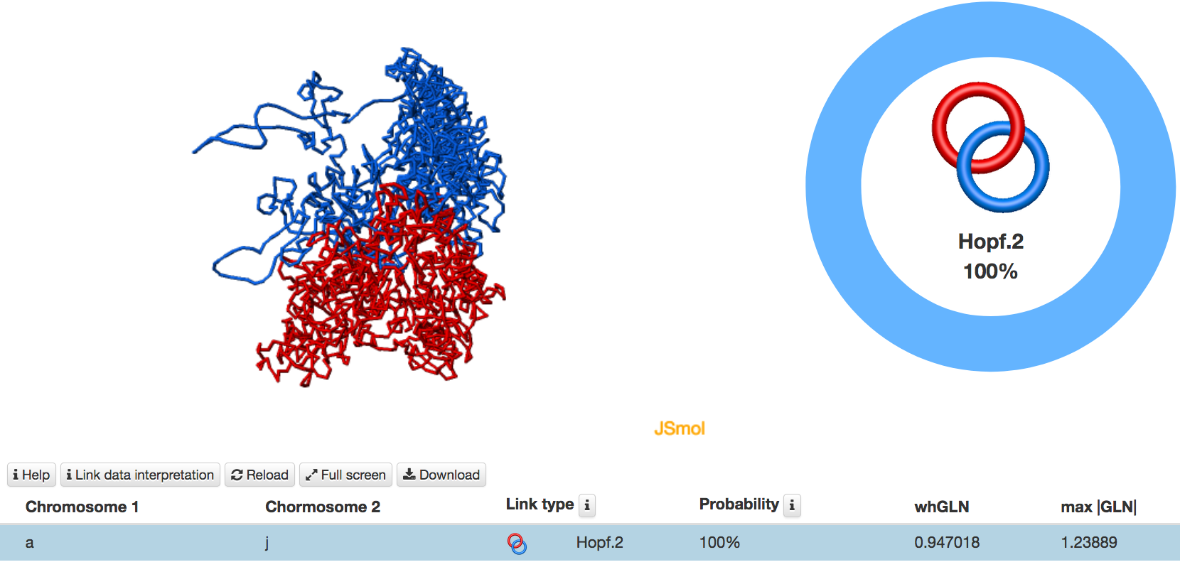
Fig. 5 Example of analysis of a pair of chromosome structures based on deterministic method. These chromosomes form a Hopf.2 link.
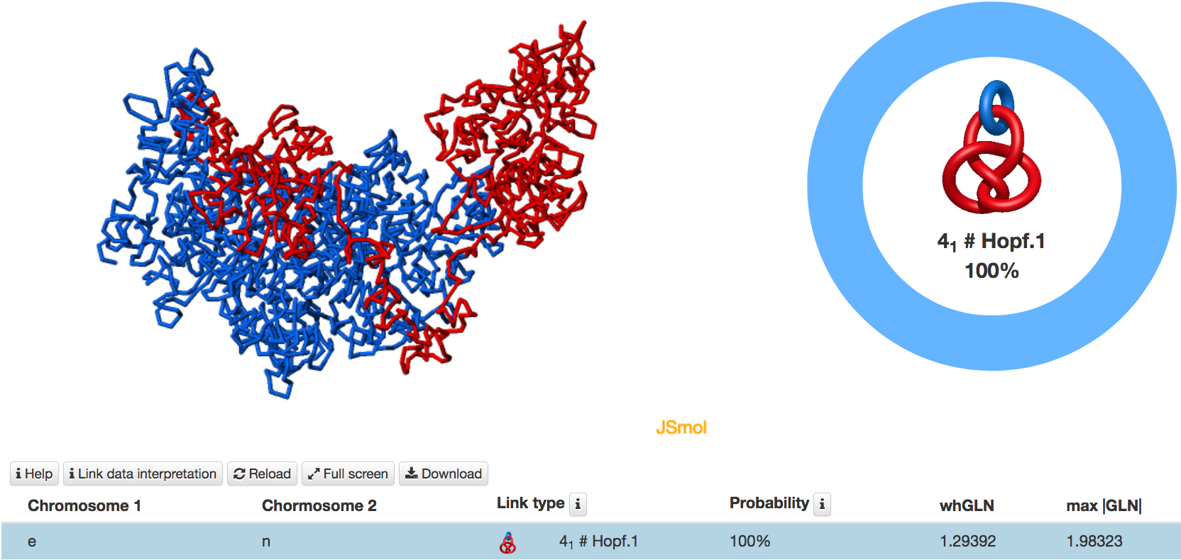
Fig. 6 Example of analysis of a pair of chromosome structures based on deterministic method. These chromosomes form a 4_1#Hopf.2 link.
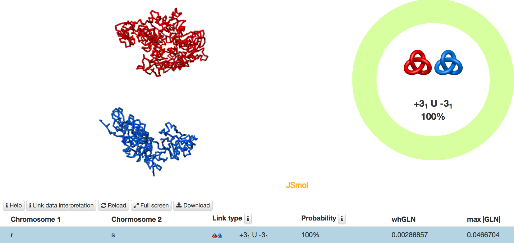
Fig. 7 An example of analysis of a pair of chromosome structures based on deterministic method. These chromosomes are unlinked, however each single chromosome forms a 31 knot.