Knots in chromosome are detected based on the method established before to study protein chains [1] with optimizations taking into account the specific properties of chromosomes. Below, we summarize the most important information and modifications to the previous algorithm (http://knotprot.cent.uw.edu.pl/knot_detection) [2] concerning knot detection in chromosomes.
Knots are the basic objects studied in the mathematical field of knot theory. Knot theory studies entanglements in closed curves, although these ideas can be extended to characterize knotting in open chains [1,2,3,4,5]. To characterize knots in chromosomes, we follow the method established by us for proteins [5].
Knots are defined uniquely on closed chains only. To define them in open chains (which have loose ends), such as chromosomes, one must choose how to connect the two loose ends in order to close the chain. Making this choice in the most optimal way is the first difficulty we have to overcome when analyzing chromosomes; various ways how to form a close loop on proteins are discussed in [5]. The methods used by KnotGenom are described here. Once this problem is addressed and an open chain is effectively transformed into a closed chain, we detect a knot type by computing polynomial knot invariants known as Alexander and HOMFLY polynomials.
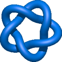
A knot can be defined by the minimal number of crossings when projected onto a plane. Thus, the simplest nontrivial knot is called trefoil (denoted also by 31). A knot with four crossings is called figure-8 (denoted by 41), knots with five crossings are denoted by 51 and 52. There are three knots with six crossings, one of them is called Stevedore's knot (denoted by 61). An unknotted loop is called the trivial knot, or the unknot, and is denoted by 01. In the notation above, the first number denotes the minimal number of crossings a given knot can show in a projection (e.g. minimal number of crossings in a projection of a trefoil onto a plane is 3). The 31, 52 and 61 knots are chiral, i.e. they differ from their mirror images, and their complete characterization requires the determination of their chirality, which we denote by a plus (+) or a minus (-) sign next to the symbol of a knot. The 41 knot is an example of an achiral knot, i.e. it is identical to its mirror image and it cannot have assigned chirality.
Knots detected in chromosomes are much more complex than those presented above; moreover, multiple knots can be identified on a single chain, and one knot can be embedded in another one. Details about knot classification used in KnotGenom are described in Knot Classification section.
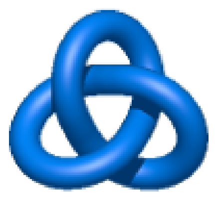
Fig. 1 Examples of prime knots.
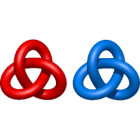
Fig. 2 Examples of composite knot 31#31. Left panel — Granny knot, right panel — square knot.
It is impossible to unambiguously define the concept of knotting for an open chain [1]. Only in the case of a closed chain the knot type is uniquely determined, and the techniques for classifying the knotting in open chains rely on closing the chain. However, for open chains the knot type can change depending on the way the chain is closed [2]. To detect knots in a long single chromosome chain we used following methods:
Fig. 3 Schematic representation of a chromosome enclosed within a large sphere with different enclosure methods used in KnotGenom. Panel A — random closure method. Panel B — the centre of mass method. Panel C — direct closure method. The enclosing sphere is represented by a black circle, and an enclosing chain fragment is depicted with the yellow line.
The knot types resulting from individual closures are determined by computing polynomial knot invariants. For quick computations of all analyzed subchains, we use the Alexander polynomial. To detect chirality of formed knots, the HOMFLY polynomial is calculated for some of the analyzed subchains.
Computing knot polynomials is relatively fast for short chains, however, it can be a very time consuming process for long chains, and chromosomes are an order of magnitude longer than a typical protein (150 amino acids, each amino acid is represented as a single bead). Thus, to compute polynomials for a given chromosome, we used a method tested before for proteins. Before computing the Alexander polynomial for a given chain (or fixed subchain), after closing terminals (for each random closure separately), we first reduce it to a shorter configuration using the KMT algorithm [2,3]. This algorithm analyzes all triangles in a chain made by three consecutive beads, and removes the middle bead if no other segment of the chain intersects with the corresponding triangle. In effect, after a number of iterations, the initial chain is replaced by a (much) shorter chain of the same topological type.
The algorithm used by the KnotGenom distinguishes knots up to 10 crossings (prime knots) and up to 12 composite knots.
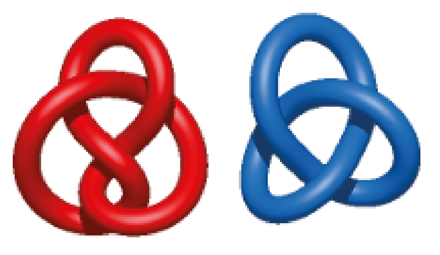
Fig. 4 Examples of composite knots found in the chromosome chains: 31 # 31 and 31 # 41.
In proteins we have found only prime knots. In contrast, our analysis of available data [2] indicates that composite knots are quite frequent in chromosomes. Below, a few examples of composite knots identified in chromosomes are presented.
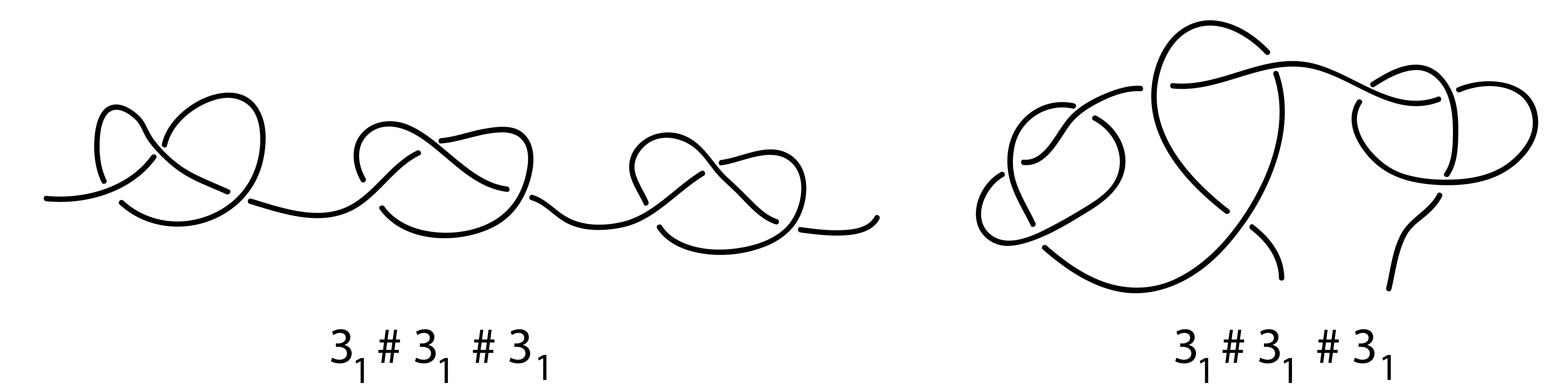
Fig. 5 Examples of different types of composite knots 31 # 31 # 31 . Left panel: three 31 prime knots, are placed separable. Right panel: three 31 prime knots, are not placed separable along the chain.
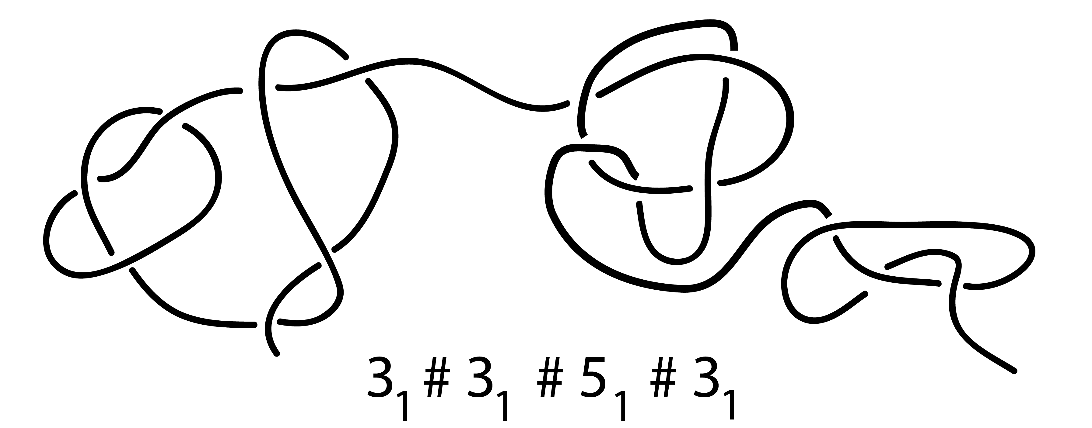
Fig. 6 An example of a complex composite knot found along the chromosome chain using KnotGenom.
| Link name | Image |
| Unknot |  |
| Trefoil +31 + and - denotes chirality. The same figures are used in both cases. |
 |
| Figure eight 41 |
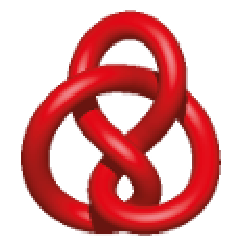 |
| +51 -51 |
 |
| ... | |
| Other Other denotes knots with more than 10 crossings. |
 |
| +31 # +31 +31 # -31 -31 # -31 -31 # +31 # denotes any composite knot. For example 31 # 31 denotes a knot made of two trefoil knots. The same figure is used for a sum of knots with different chirality. |
 |
| ... | |
| +31 # 41 41 # +31 The same figure is used for the sum of two composite knots composed of the same type of knot. The knots are ordered from the most complex to the simplex one |
 |
|
31 # 31 # 31
Composite knots composed of more than 3 prime knots are represented with a graphic. |
No figure Such figure is too complex to be well visualized. |
| +31 # Other
Example of a composite knot, sum of trefoil knot and knot with more than 10 crossings. |
|