Interpreting knotting data

The user can upload and analyze two types of data: either a single chromosome, or the whole cell. In this section we explain how to identify entangled structures along a single chain (a chromosome, or any other polymer-like chain with similar size): knots and slipknots.

Knot analysis can be conducted based on random, centre of mass, or direct closure methods, on two different levels:

  • detailed - a full topological fingerprint is determined
  • general - entanglement of the whole chain is determined

Moreover, the user can use all these methods together with the relaxation procedure to estimate entanglement stability [1].


Entanglements of a single chromosomes are presented in the following manner. The information displayed from top to bottom of the result page can be divided into:

Each of these parts is described in detail below.

Examples


Interpreting job status

At the top of the page, the first tab indicates the status of a submitted job, as shown in Fig 1. The tab summarizes options used by the user to submit a job. The most important information is:

  • The success of calculation is indicated by its Status: Finished (in green) or unsuccessful (in red).
  • Results - informs the user whether a knot has been indentified.
  • Chain closing method - informs the user about the method used to close the chromosome chain. For a random closure method, the number of random points is shown.

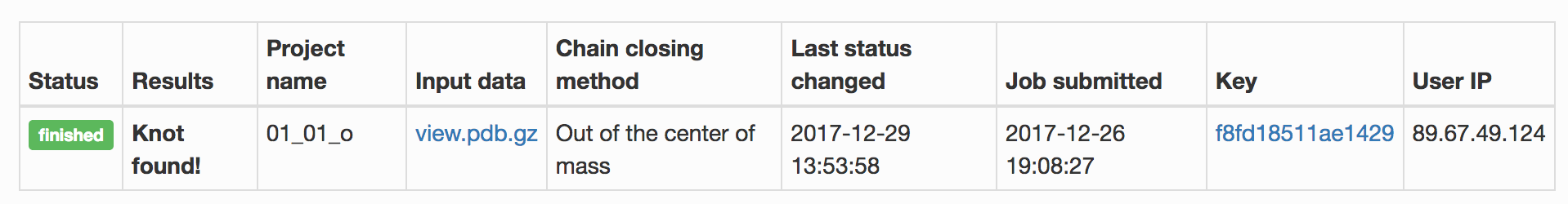
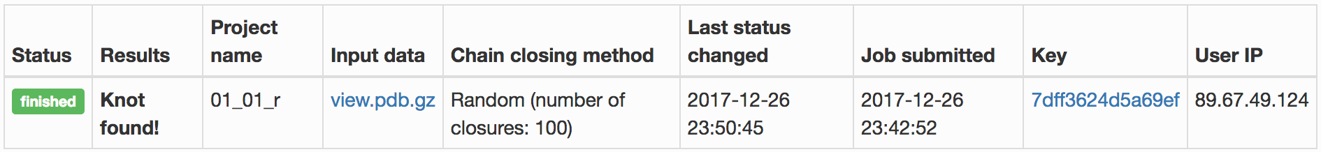
Fig. 1 Example of the job results page – interpretation of job status. Panels from top to bottom show the top of the results page for three different methods used to close the chromosome: out of the centre mass, direct, and random closure method. The last panel shows the results page for a job that is still running, when some data is already available in a form of a topological fingerprint even though the relaxation method is still running.

Users can name their jobs, hide them on the job queue, and, by supplying their e-mail addresses, request to be notified when their job finishes. E-mail addresses are stored only until the job finishes, all other data about the jobs is stored for two weeks.


Graphical representation of entanglement of a chromosome

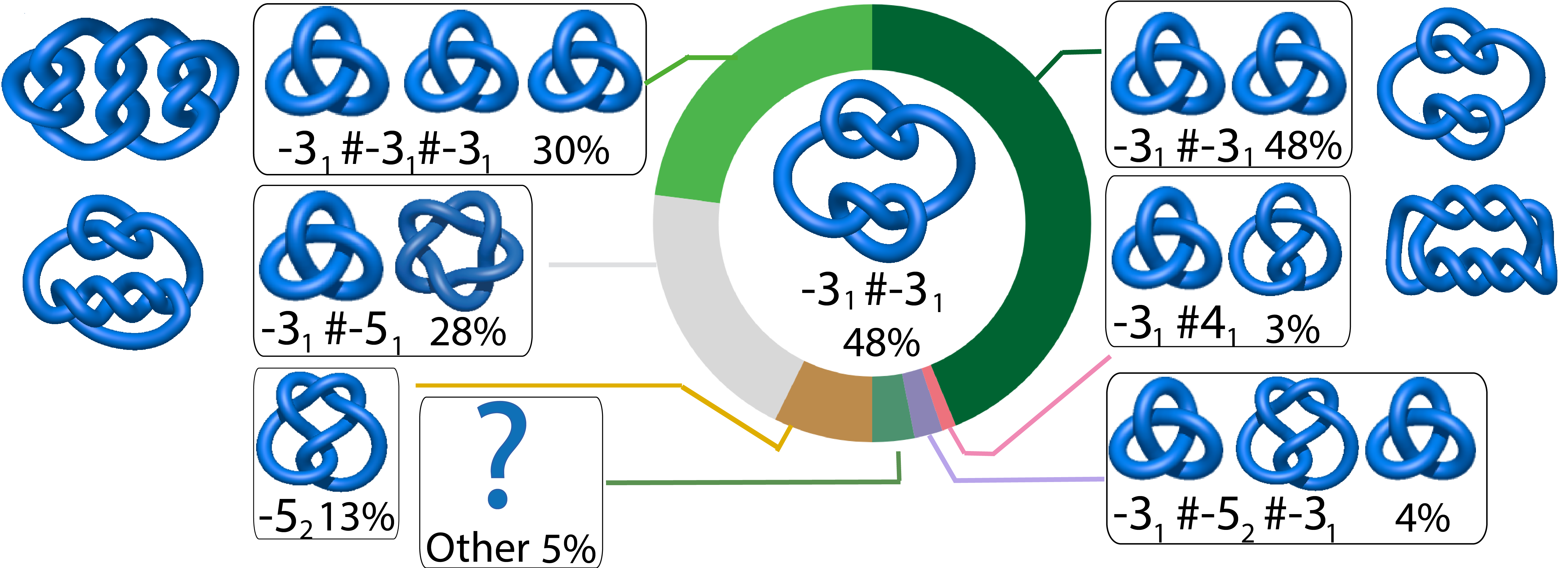
In the most advanced option critical information about the knot type and its likelihood is presented using four methods:

  • an interactive matrix, which shows all knots and slipknots - a fingerprint option
  • interactive pie chart – the main type option
  • a table with detailed information about the most probable knots (all options) and slipknots - a fingerprint option
  • graphical representation of the above data directly on the chromosome chain - a fingerprint option

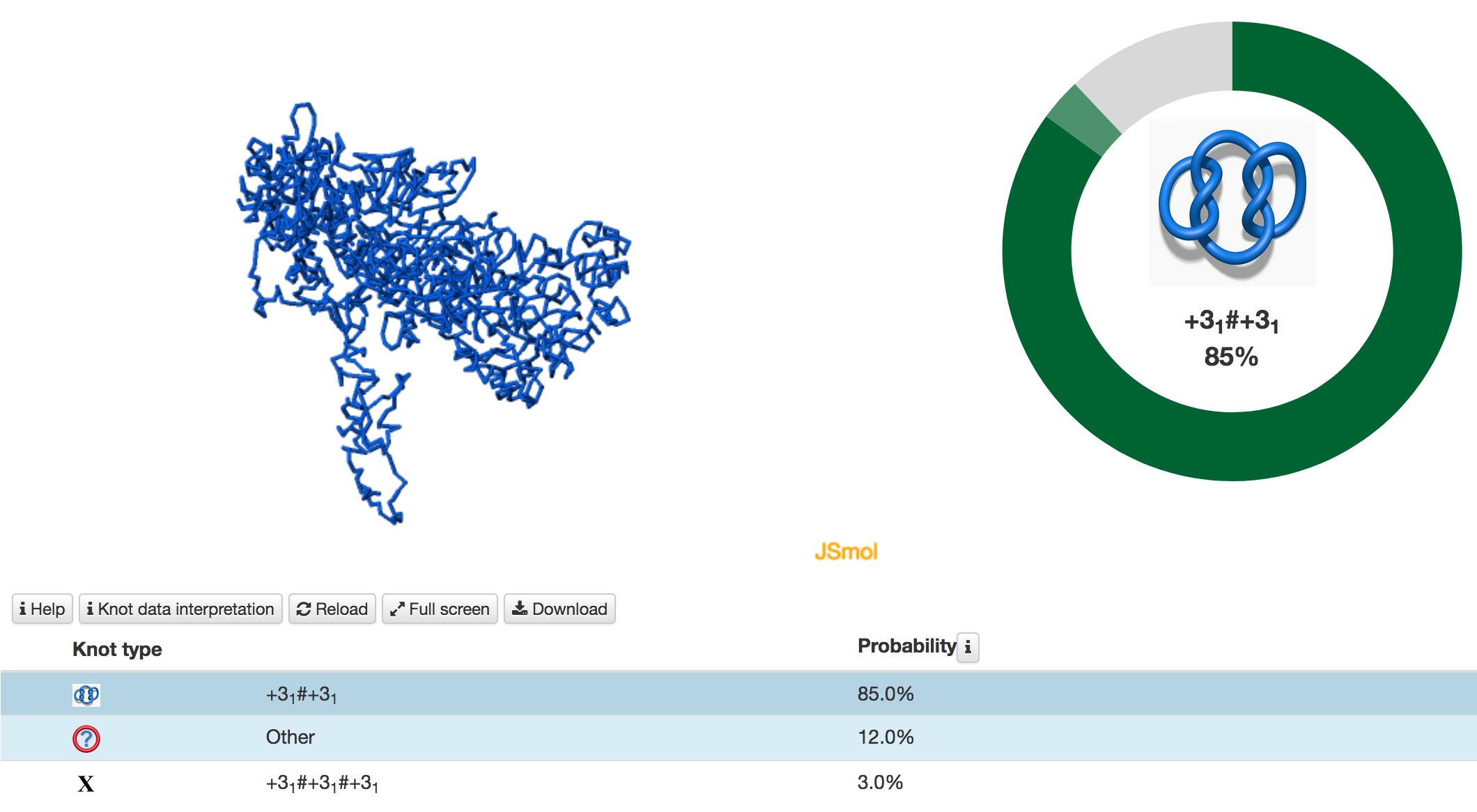
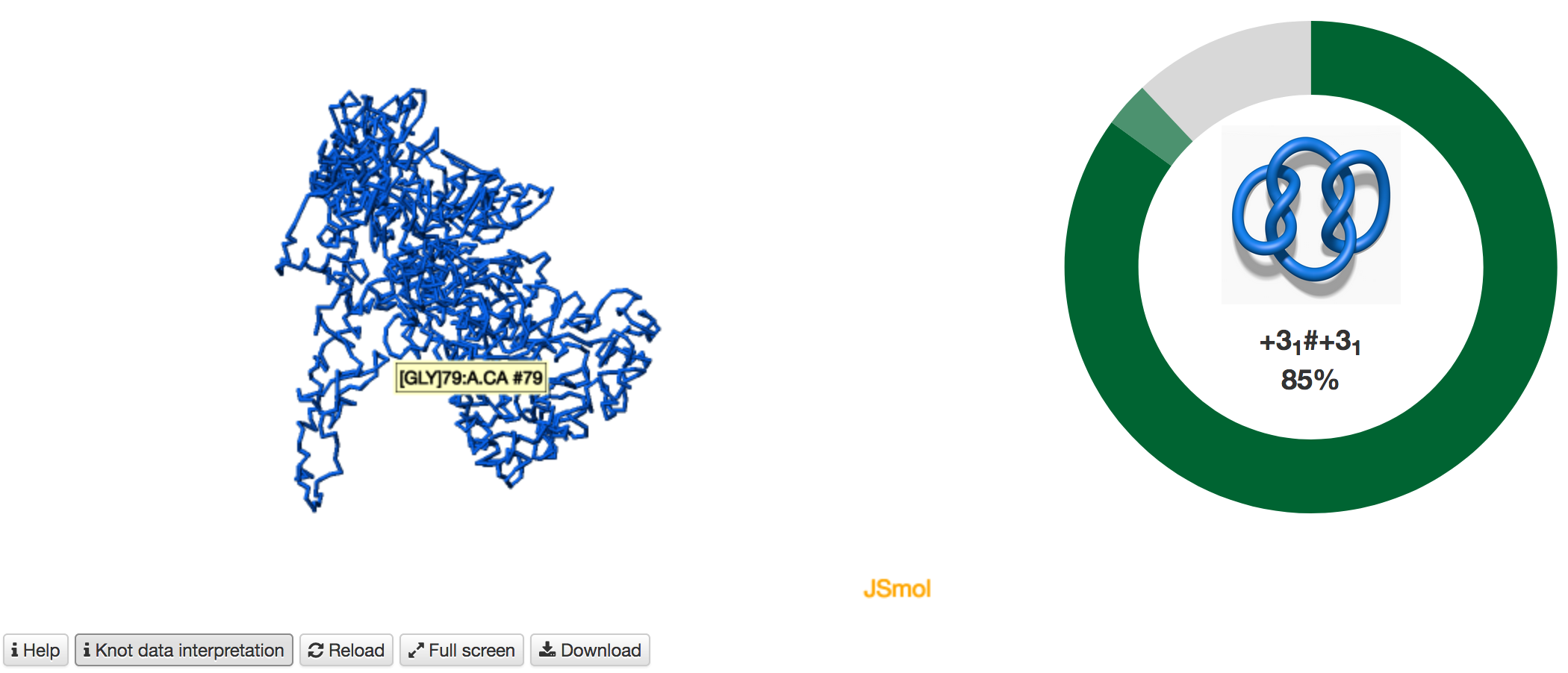
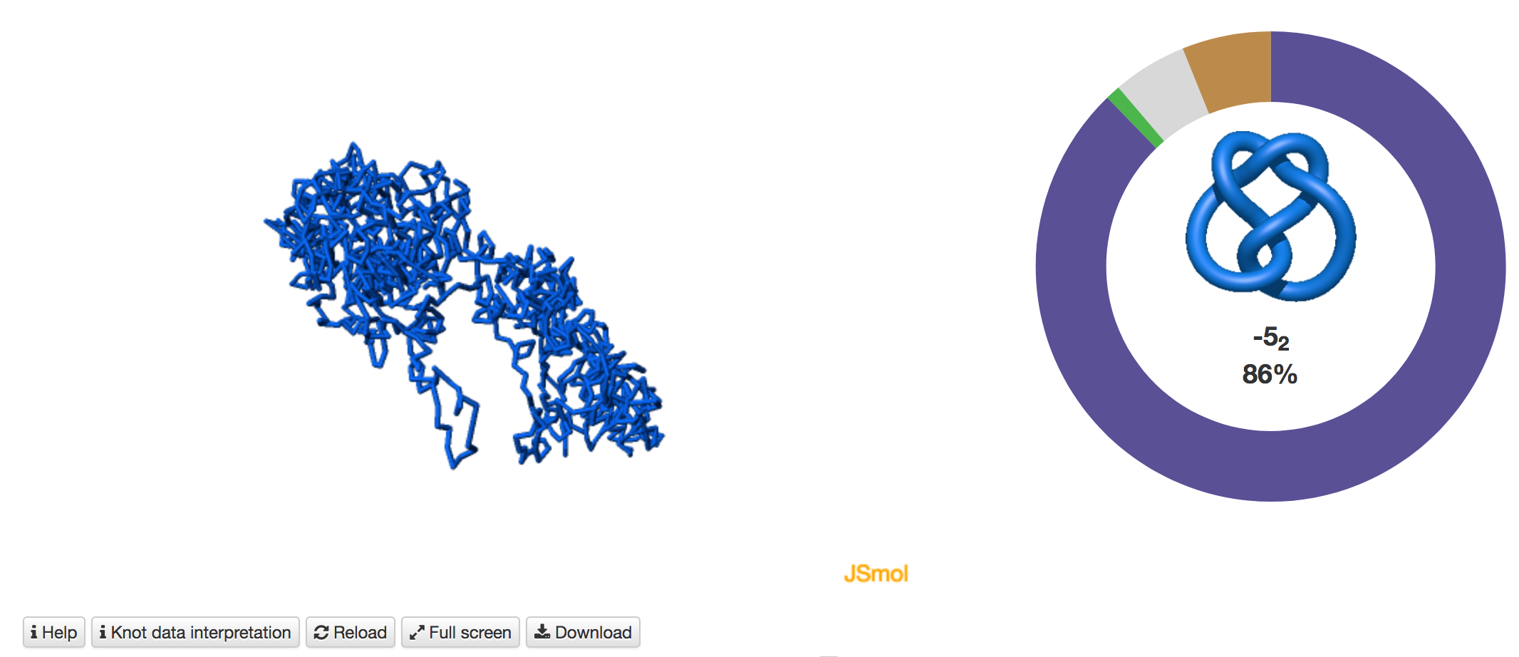
The main part of the default page contains the JSmol presentation of the chromosome structure and one of the two graphical representations:

  • the topological fingerprint (left) representing the comprehensive information about entanglement of a given structure – e.g. Fig. 2. The fingerprint is presented in the form of a matrix diagram that shows users the knot type of the entire chromosome chain and of each of its subchains. The "knotting fingerprint of a chromosome" encodes information about locations of the "knot core", "knot tails", "slipknot loops", and "slipknot tails", whose definitions are given here. When the random closure method is used the intensity of color represents a probability of detecting a given knot (knots are detected only with some probability, which is a consequence of a choice of their closure, as explained in section Knot detection). The probability is normalized and shown in the table below the plot. When the centre of mass, or the direct closure method is used, the total probability always equals 100%, since there is only one closure. The figure below presents an example of a knotting fingerprint, which in this case contains an area representing a single slipknot. The same information is also shown in a graphical form (in JSmol), right.

    Fig. 2 Example of the job results page when a matrix fingerprint is determined using the random closure method. For each knot type observed, the corresponding topological and geometrical data is shown on the chromosome structure and listed in the table in the light blue row.

  • pie chart with basic information. When the user choses the Main type option, only entanglement of the full length of the chromosome is determined. In this case the random closure method identifies the most probable knot type and also the likelihood of forming other knots. The probability of forming other knots is presented using an interactive pie chart (Fig. 3). Moreover, for each knot type observed, the corresponding topological and geometrical data are shown on the chromosome structure. This option enables the user to analyze knots of some particular interest.

    Fig. 3 The pie chart representing the likelihood of the knots identified. An example of a pie chart when random closure method is used. In the case of the random closure method by default, the most probable knot is shown in the center of the plot. Upon placing the cursor over a region of the chart, the corresponding knot and its likelihood are displayed in the center of the pie chart. The symbol # denotes the composite knot, the sum of the prime knots.


A table summarizing detected entangled elements

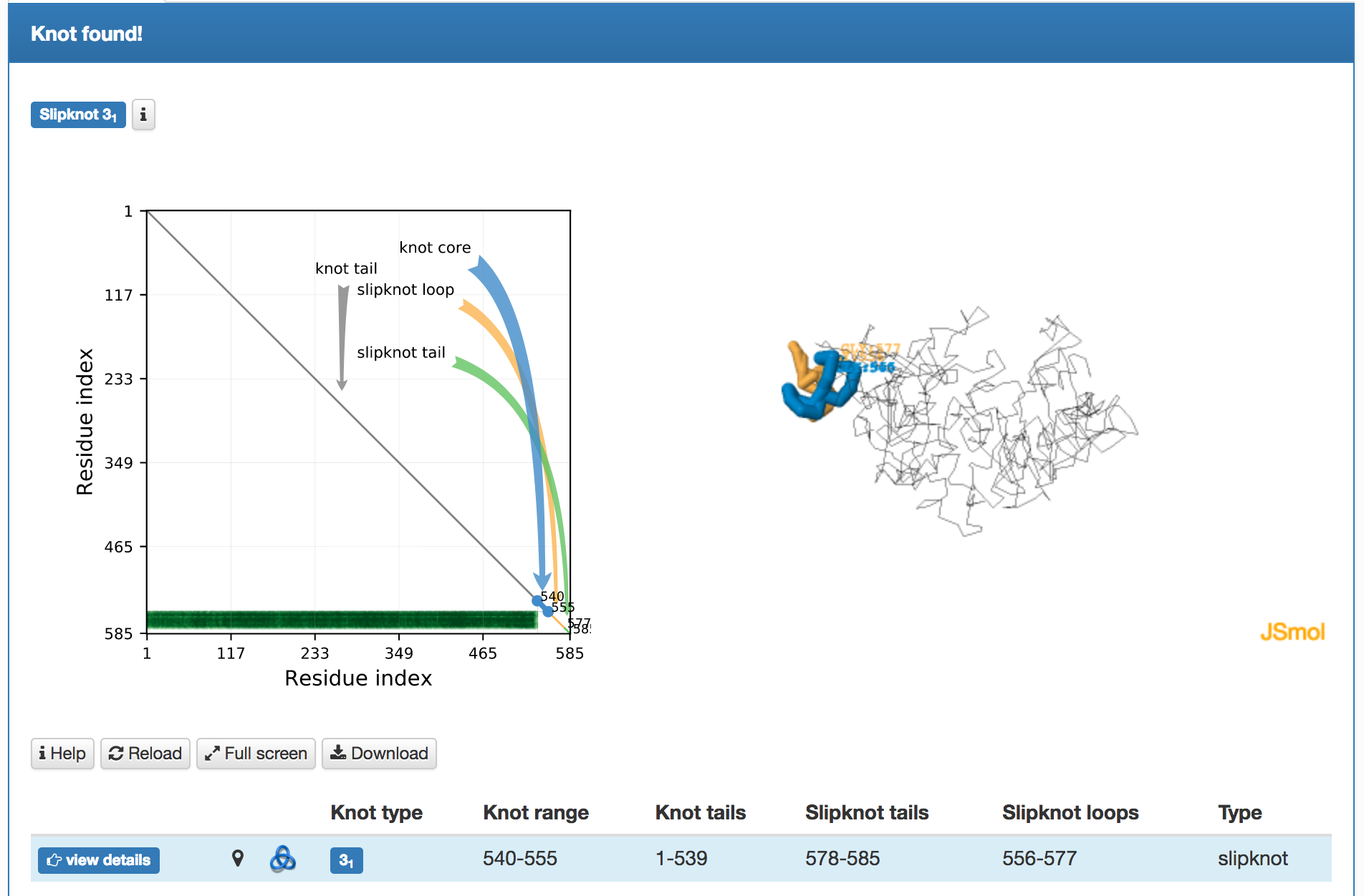
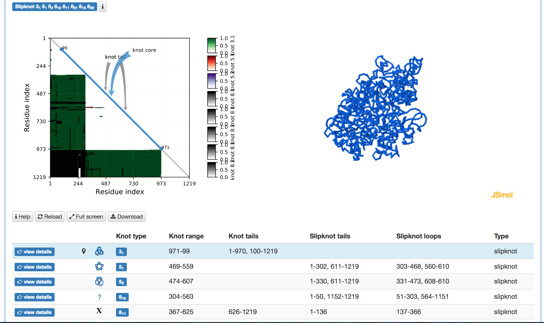
The topological and structural details about the most probable knots are stored in the table below the graphical presentation (Fig.4). Each row of the table corresponds to one knot. The rows are sorted with decreasing likelihood of the knot topology. In each row, one can find the minature depiction of the knot identified along with its name and likelihood. The rest of the table presents position of the knot core, slipknot loop, the knot tails. All this information is visible in the JSmol presentation.

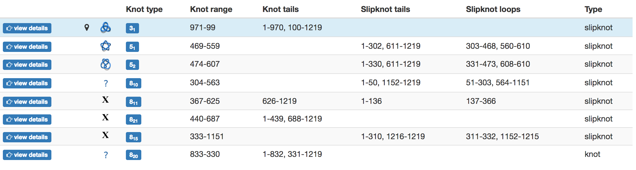
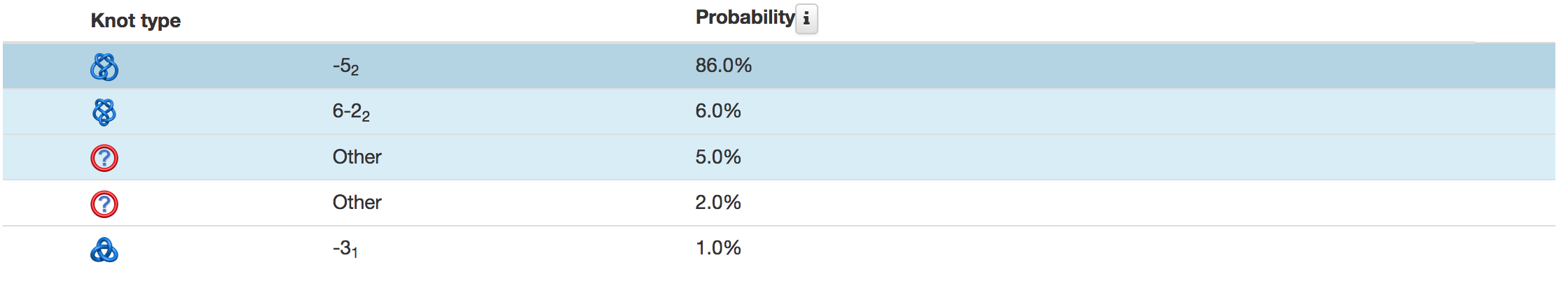
Fig. 4 Example of the table showing the observed knots in the case of the random and the direct closure method are shown in the top and bottom panel, respectively. In the case of the random closure method, the table shows detailed data about knots and slipknots type and position formed by backbone subchains. In the case of the direct closure method the table shows the knot type and probability of all identified knots.


Relaxation - robustness of the topology

The relaxation method is used to estimate the robustness of the topology of a given chromosome. The change in the conformation of the chromosome is investigated via molecular dynamics (it is described here) and a criterion to determine the robustness of topology is described here. The data for relaxation (Fig. 5) is presented as follows:

  • The main result - robustness of the topology
  • Detailed description of temporary topology

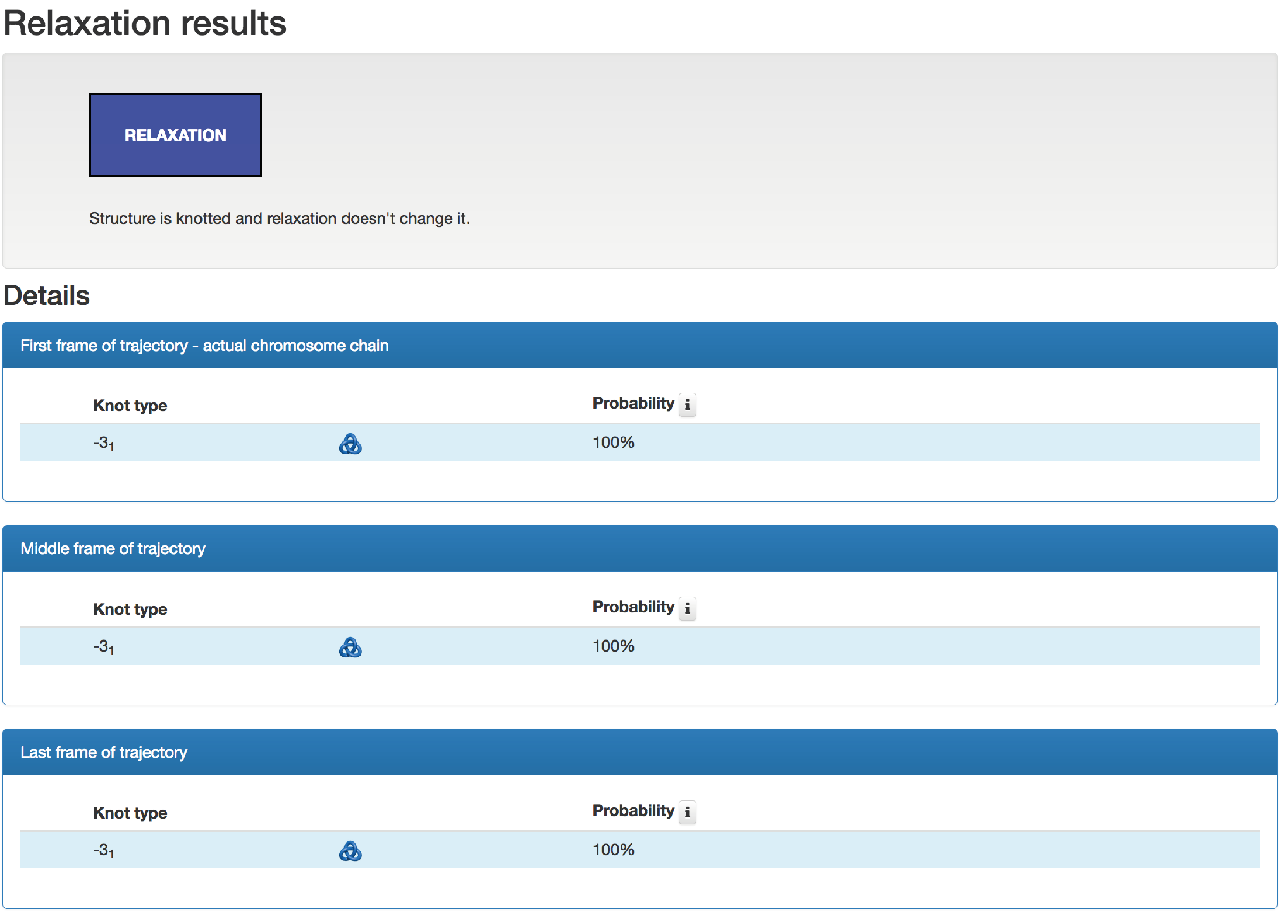
Fig. 5 Overview of the result page for a single chromosome relaxation analysis. This data shows that a sample knot remains conserved during the whole simulation.

Main result

The result of relaxation - the robustness of an investigated topology - is described via four colors and presented at the top of the page in the box called "Relaxation results":

  • White - Structure is Unknotted / Unlinked and relaxation does Not Change it,
  • Blue - Structure is Knotted / Linked and relaxation does Not Change it,
  • Orange - Structure is Knotted / Linked, and after relaxation it is Unknotted / Unlinked,
  • Red - Relaxation Changes the type of entanglement of the structure.

Detailed description of temporary topology

The robustness of the topology is estimated based on the type of the topology identified in temporary conformations. The table below presents details about identified topologies in the original conformation, and middle and last frames, which were used to estimate the robustness of topology. The table contains the knot type, its schematic drawing, and probability of identified topology.


Examples

Fig. 6 Example of the job results pages when the user chooses the Main type option. In this case, only the entanglement of the full length of a chromosome is determined. When the random closure method is additionally used, KnotGenom identifies the most probable knot type and also the likelihood of forming other knots. The likelihood is shown on the right. Please note that when the minature depiction (figure) of the knot is very complex, and we thus do not have a corresponding picture, it is denoted with X.


[1] JT Siebert, AN Kivel, LP Atkinson, TJ Stevens, ED Laue, P Virnau, Are There Knots in Chromosomes? Polymers (2017)
[2] Stevens, T.J.; Lando, D.; Basu, S.; Atkinson, L.P.; Cao, Y.; Lee, S.F.; Leeb, M.; Wohlfahrt, K.J.; Boucher, W.; O’Shaughnessy-Kirwan, A.; et al. 3D structures of individual mammalian genomes studied by single-cell Hi-C. Nature 2017, 544, 59-64.


KnotGenom | Interdisciplinary Laboratory of Biological Systems Modelling